作品として見る 生成された文書そのもの — 切り替えも開閉もそのまま動きます
作品として見る 生成された文書そのもの — 切り替えも開閉もそのまま動きます
コピーして貼るか、ファイルに保存して渡す。ネットにつながらない環境には「全部入り」を 1 つ渡せば足りる。
このパネルの中身を、URL の先にあるファイルの中身まで含めて 1 つにまとめた Markdown — 大きいのでファイルで渡す(コピーは 32KB まで)
「予測確率の校正曲線」でHTML資料を作ってください。この型は実行できるので、版面を組み直す必要はありません — 必要なのは中身です。

## この型がすること
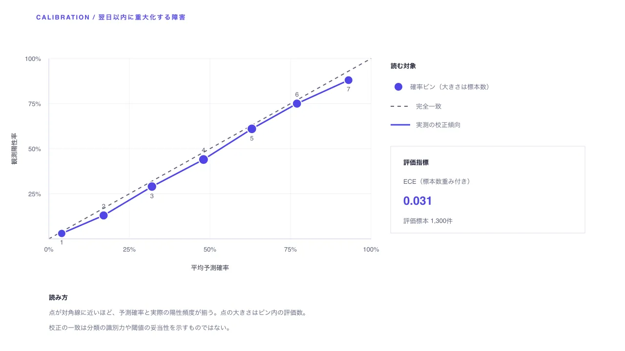
予測確率を区間化し、各区間の平均予測確率と観測陽性率を完全一致の対角線に照らして信頼性を読む。

## 渡す必要があるもの
- 陽性クラスと評価標本総数を示す。
- 0〜1を隙間・重複なく覆う4〜12区間を昇順で指定し、各区間の平均予測確率・観測陽性率・標本数を入力する。標本数合計は総数と一致させる。

## 入力の形
- `title` — string — 予測確率の信頼性について伝える見出し
- `subtitle` — string? — 評価データ・対象期間・分割条件
- `positiveClass` — string — 確率として予測した陽性イベント
- `evaluationCount` — integer — 全ビンの評価標本数
- `bins` — array (id, label, lowerBound, upperBound, predictedMean, observedRate, sampleCount) — 4〜12区間。確率値は0〜1、区間連続、予測平均は範囲内、標本数合計は総数と一致

入力の機械可読な検証は schema.ts が持ちます。足りない入力は推測せず質問してください。

## 向かない場合
- 閾値を動かしたときの偽陽性率・真陽性率や識別順位を見る場合はROC曲線を使う。
- 同じ指標を持つ一般の観測対象同士の関係を見る場合は散布図を使う。校正は予測値と実現頻度の対応に限る。

## 作り方
入力を JSON にまとめ、次を実行します。

```bash
node scripts/render.mjs calibration-curve <入力.json> --theme ink -o out.html
```

出力は 1 ファイルで完結し、外部から何も読み込みません。

## 原本
- https://design-vault.pages.dev/designs/calibration-curve/source/template.tsx
- https://design-vault.pages.dev/designs/calibration-curve/source/schema.ts
- https://design-vault.pages.dev/designs/calibration-curve/source/sample-data.json
- https://design-vault.pages.dev/designs/calibration-curve/sample.html
テンプレート・入力スキーマ・サンプルデータ・メタ情報。この文書はこの 4 つから生成されています。 生成された文書
/designs/calibration-curve/source/template.tsx
import type { Props } from "./schema";

const CSS = ".asset{font-family:var(--font-sans);color:var(--color-on-surface);background:var(--color-surface);max-width:var(--container-slide);margin:auto;padding:2.5rem 3rem;line-height:1.5}.asset *{box-sizing:border-box}.asset h1{font-size:var(--text-h1);line-height:1.3;margin:0}.asset .subtitle{color:var(--color-secondary);margin:.6rem 0 1.25rem}.asset .eyebrow{font:600 var(--text-label) var(--font-mono);letter-spacing:.1em;color:var(--color-tertiary)}.asset .plot{display:block;width:100%;height:auto}.asset .summary{display:grid;grid-template-columns:repeat(3,minmax(0,1fr));gap:1rem;margin:1rem 0 1.5rem}.asset .metric{padding:1rem;background:var(--color-surface-subtle);border-top:3px solid var(--color-tertiary);min-width:0}.asset .metric dt{font-size:var(--text-label);color:var(--color-secondary)}.asset .metric dd{margin:.25rem 0 0;font:700 var(--text-h2) var(--font-mono);overflow-wrap:anywhere}.asset .ledger{border-collapse:collapse;width:100%;font-variant-numeric:tabular-nums}.asset .ledger th,.asset .ledger td{text-align:left;vertical-align:top;padding:.65rem .75rem;border-bottom:1px solid var(--color-outline);overflow-wrap:anywhere}.asset .ledger th{color:var(--color-secondary)}.asset .ledger .mono{font-family:var(--font-mono)}.asset details{margin-top:1rem}.asset summary{cursor:pointer;min-height:2.75rem;padding:.5rem 0;color:var(--color-secondary)}.asset .note{border-left:3px solid var(--color-outline);padding:.75rem 1rem;color:var(--color-secondary)}@media(max-width:640px){.asset{padding:1.5rem 1rem}.asset h1{font-size:var(--text-h2)}.asset .summary{grid-template-columns:1fr}.asset .ledger,.asset .ledger tbody,.asset .ledger tr,.asset .ledger td{display:block}.asset .ledger thead{display:none}.asset .ledger tr{padding:.65rem 0;border-bottom:1px solid var(--color-outline)}.asset .ledger td{display:grid;grid-template-columns:9rem minmax(0,1fr);gap:.75rem;border:0;padding:.2rem 0}.asset .ledger td:before{content:attr(data-label);font-size:var(--text-label);color:var(--color-secondary)}}";
const fmt = (value: number) => Math.round(value * 100) + "%";
const fmtDelta = (value: number) => (value * 100).toFixed(1) + "pp";
const ece = (d: Props) => d.bins.reduce((sum, bin) => sum + bin.sampleCount * Math.abs(bin.observedRate - bin.predictedMean), 0) / d.evaluationCount;
const curvePath = (d: Props) => d.bins.map((bin, index) => (index ? "L " : "M ") + (100 + bin.predictedMean * 660) + " " + (490 - bin.observedRate * 370)).join(" ");

export default function Template(d: Props) {
  const error = ece(d);
  const maxCount = Math.max(...d.bins.map(bin => bin.sampleCount));
  const tick = [0, .25, .5, .75, 1];
  return <section className="asset asset-calibration-curve">
    <style>{CSS}</style>
    <header><p className="eyebrow">CALIBRATION CURVE / PREDICTED VS OBSERVED</p><h1>{d.title}</h1>{d.subtitle && <p className="subtitle">{d.subtitle}</p>}</header>
    <svg className="plot" data-layout-still="true" width="1280" height="720" viewBox="0 0 1280 720" role="img" aria-labelledby="calibration-title calibration-desc" fontFamily="sans-serif" fontSize="13" fill="var(--color-secondary)">
      <title id="calibration-title">{d.title}</title>
      <desc id="calibration-desc">{d.positiveClass}の予測確率と観測率の関係。対角線は完全一致。標本数で重み付けした絶対確率誤差ECEは {error.toFixed(3)}、評価標本数は{d.evaluationCount}件。</desc>
      <rect x="0" y="0" width="1280" height="720" fill="var(--color-surface)" />
      <text x="74" y="40" fontSize="13" fontWeight="700" letterSpacing="2" fill="var(--color-tertiary)">CALIBRATION / {d.positiveClass}</text>
      {tick.map((value, index) => {
        const x = 100 + value * 660, y = 490 - value * 370;
        return <g key={index}>
          <line x1="100" y1={y} x2="760" y2={y} stroke="var(--color-outline)" strokeWidth="1" opacity=".48" />
          <line x1={x} y1="120" x2={x} y2="490" stroke="var(--color-outline)" strokeWidth="1" opacity=".48" />
          <text x={x} y="516" textAnchor="middle">{fmt(value)}</text>{value > 0 && <text x="84" y={y + 5} textAnchor="end">{fmt(value)}</text>}
        </g>;
      })}
      <line x1="100" y1="490" x2="760" y2="120" stroke="var(--color-secondary)" strokeWidth="2" strokeDasharray="7 7" />
      <path d={curvePath(d)} fill="none" stroke="var(--color-tertiary)" strokeWidth="3" strokeLinejoin="round" />
      {d.bins.map((bin, index) => {
        const cx = 100 + bin.predictedMean * 660;
        const cy = 490 - bin.observedRate * 370;
        const radius = 5 + Math.sqrt(bin.sampleCount / maxCount) * 5;
        const labelX = index === 10 ? cx + 18 : cx;
        const labelY = index === 10 ? cy - 18 : cy + (index % 2 === 0 ? radius + 14 : -radius - 5);
        return <g key={bin.id} data-calibration-bin={bin.id}>
          <circle cx={cx} cy={cy} r={radius} fill="var(--color-tertiary)" stroke="var(--color-surface)" strokeWidth="2" />
          <text x={labelX} y={labelY} textAnchor="middle">{index + 1}</text>
        </g>;
      })}
      <line x1="100" y1="490" x2="760" y2="490" stroke="var(--color-outline)" strokeWidth="1.5" /><line x1="100" y1="120" x2="100" y2="490" stroke="var(--color-outline)" strokeWidth="1.5" />
      <text x="430" y="554" textAnchor="middle" fill="var(--color-on-surface)">平均予測確率</text><text x="34" y="305" textAnchor="middle" transform="rotate(-90 34 305)" fill="var(--color-on-surface)">観測陽性率</text>
      <text x="800" y="140" fontWeight="700" fill="var(--color-on-surface)">読む対象</text><circle cx="816" cy="178" r="8" fill="var(--color-tertiary)" /><text x="840" y="183">確率ビン(大きさは標本数)</text>
      <line x1="800" y1="218" x2="840" y2="218" stroke="var(--color-secondary)" strokeWidth="2" strokeDasharray="7 7" /><text x="852" y="223">完全一致</text>
      <line x1="800" y1="256" x2="840" y2="256" stroke="var(--color-tertiary)" strokeWidth="3" /><text x="852" y="261">実測の校正傾向</text>
      <rect x="800" y="300" width="398" height="178" fill="var(--color-surface)" stroke="var(--color-outline)" />
      <text x="826" y="338" fontWeight="700" fill="var(--color-on-surface)">評価指標</text><text x="826" y="377">ECE(標本数重み付き)</text>
      <text x="826" y="420" fontSize="24" fontWeight="700" fill="var(--color-tertiary)">{error.toFixed(3)}</text><text x="826" y="458">評価標本 {d.evaluationCount.toLocaleString("ja-JP")}件</text>
      <text x="100" y="615" fontWeight="700" fill="var(--color-on-surface)">読み方</text>
      <text x="100" y="646">点が対角線に近いほど、予測確率と実際の陽性頻度が揃う。点の大きさはビン内の評価数。</text>
      <text x="100" y="677">校正の一致は分類の識別力や閾値の妥当性を示すものではない。</text>
    </svg>
    <dl className="summary">
      <div className="metric"><dt>ECE|標本数重み付き絶対誤差</dt><dd>{error.toFixed(3)}</dd></div>
      <div className="metric"><dt>評価対象の陽性クラス</dt><dd>{d.positiveClass}</dd></div>
      <div className="metric"><dt>評価標本数</dt><dd>{d.evaluationCount.toLocaleString("ja-JP")}件</dd></div>
    </dl>
    <p className="note">ECEはビン集約に依存する校正誤差です。校正結果だけから識別性能・閾値・個別予測の妥当性を結論しないでください。</p>
    <details open><summary>各確率ビンと予測・観測値を確認({d.bins.length}区間)</summary>
      <table className="ledger"><thead><tr><th>番号 / 確率区間</th><th>平均予測</th><th>観測陽性率</th><th>標本数</th><th>校正差(観測−予測)</th></tr></thead>
        <tbody>{d.bins.map((bin, index) => <tr key={bin.id} data-calibration-bin={bin.id}>
          <td data-label="確率区間">{index + 1} / {bin.label}({fmt(bin.lowerBound)}–{fmt(bin.upperBound)})</td>
          <td data-label="平均予測" className="mono">{fmt(bin.predictedMean)}</td><td data-label="観測陽性率" className="mono">{fmt(bin.observedRate)}</td>
          <td data-label="標本数" className="mono">{bin.sampleCount.toLocaleString("ja-JP")}</td><td data-label="校正差" className="mono">{bin.observedRate >= bin.predictedMean ? "+" : ""}{fmtDelta(bin.observedRate - bin.predictedMean)}</td>
        </tr>)}</tbody>
      </table>
    </details>
  </section>;
}
/designs/calibration-curve/source/schema.ts
import { z } from "zod";

const text = z.string().trim().min(1).max(160);
const label = z.string().trim().min(1).max(64);
const id = z.string().trim().min(1).max(24);
const probability = z.number().finite().min(0).max(1);

export const schema = z.object({
  title: text.describe("予測確率の信頼性について伝える見出し"),
  subtitle: text.optional().describe("評価データ・対象期間・分割条件"),
  positiveClass: label.describe("確率として予測した陽性イベント"),
  evaluationCount: z.number().int().positive().describe("全確率ビンに含まれる評価標本数"),
  bins: z.array(z.object({
    id: id.describe("確率ビンの一意なID"),
    label: label.describe("確率範囲や評価対象を識別する説明"),
    lowerBound: probability.describe("予測確率ビンの下端を含む"),
    upperBound: probability.describe("予測確率ビンの上端。次のビンの下端と一致する"),
    predictedMean: probability.describe("ビン内の平均予測確率"),
    observedRate: probability.describe("ビン内で観測された陽性割合"),
    sampleCount: z.number().int().positive().describe("ビンの評価標本数。点の大きさと重み付き誤差に使う"),
  }).strict()).min(4).max(12).describe("0〜1を分割する連続した確率ビン。4〜12区間"),
}).strict().superRefine((data, ctx) => {
  const ids = data.bins.map(bin => bin.id);
  if (new Set(ids).size !== ids.length) {
    ctx.addIssue({ code: "custom", path: ["bins"], message: "確率ビンIDは一意" });
  }
  if (data.bins.length === 0) return;
  if (data.bins[0].lowerBound !== 0 || data.bins[data.bins.length - 1].upperBound !== 1) {
    ctx.addIssue({ code: "custom", path: ["bins"], message: "確率ビンは0から1までを覆う" });
  }
  for (let index = 0; index < data.bins.length; index += 1) {
    const bin = data.bins[index];
    if (bin.lowerBound >= bin.upperBound) {
      ctx.addIssue({ code: "custom", path: ["bins", index], message: "各ビンは正の幅を持つ" });
    }
    if (bin.predictedMean < bin.lowerBound || bin.predictedMean > bin.upperBound) {
      ctx.addIssue({ code: "custom", path: ["bins", index, "predictedMean"], message: "平均予測確率は所属ビン内にある" });
    }
    if (index > 0) {
      const previous = data.bins[index - 1];
      if (Math.abs(previous.upperBound - bin.lowerBound) > 1e-9) {
        ctx.addIssue({ code: "custom", path: ["bins", index, "lowerBound"], message: "確率ビンの間に隙間や重複を作らない" });
      }
      if (bin.predictedMean < previous.predictedMean) {
        ctx.addIssue({ code: "custom", path: ["bins", index, "predictedMean"], message: "平均予測確率はビン順に非減少" });
      }
    }
  }
  if (data.bins.reduce((sum, bin) => sum + bin.sampleCount, 0) !== data.evaluationCount) {
    ctx.addIssue({ code: "custom", path: ["evaluationCount"], message: "ビン標本数の合計と評価標本数を一致させる" });
  }
});

export type Props = z.infer<typeof schema>;
/designs/calibration-curve/source/meta.yaml
id: calibration-curve
name:
  ja: 予測確率の校正曲線
  en: Probability Calibration Curve
purpose:
  ja: 予測確率を区間化し、各区間の平均予測確率と観測陽性率を完全一致の対角線に照らして信頼性を読む。
  en: Compare binned mean predicted probabilities with observed positive rates against the perfect-calibration diagonal.
status: published
still: ./still.png
category: analysis
catalogOrder: 850
jobs:
  - measure-change
  - prioritize-diagnose
useCases:
  - kpi
  - prioritization
layoutKinds:
  - matrix
tags:
  - calibration-curve
  - probability-reliability
  - model-evaluation
  - offline
  - responsive
whenToUse:
  - ja: 予測確率20%の集合で、実際にイベントが起きる割合も約20%か確認する。
    en: Use to check whether groups predicted at a given probability experience the event at a similar rate.
  - ja: 信頼度が低い確率帯を見つけ、確率補正や追加データ収集の候補を絞る。
    en: Use to find poorly calibrated probability ranges and focus recalibration or data collection.
avoidWhen:
  - ja: 閾値を動かしたときの偽陽性率・真陽性率や識別順位を見る場合はROC曲線を使う。
    en: Use an ROC curve to inspect threshold-dependent false-positive and true-positive rates or ranking discrimination.
  - ja: 同じ指標を持つ一般の観測対象同士の関係を見る場合は散布図を使う。校正は予測値と実現頻度の対応に限る。
    en: Use a scatter plot for general relationships; calibration is specifically about predicted probabilities versus realized frequencies.
requiredInputs:
  - ja: 陽性クラスと評価標本総数を示す。
    en: Define the positive class and total evaluation sample count.
  - ja: 0〜1を隙間・重複なく覆う4〜12区間を昇順で指定し、各区間の平均予測確率・観測陽性率・標本数を入力する。標本数合計は総数と一致させる。
    en: Supply four to twelve ordered contiguous bins covering zero to one, with mean predicted probability, observed positive rate, and sample count; counts must sum to the evaluation total.
relatedLayouts:
  - roc-curve
  - scatter-relationship
  - interval-estimates
dataSchema:
  title: string — 予測確率の信頼性について伝える見出し
  subtitle: string? — 評価データ・対象期間・分割条件
  positiveClass: string — 確率として予測した陽性イベント
  evaluationCount: integer — 全ビンの評価標本数
  bins: array (id, label, lowerBound, upperBound, predictedMean, observedRate, sampleCount) — 4〜12区間。確率値は0〜1、区間連続、予測平均は範囲内、標本数合計は総数と一致
sources: []
/designs/calibration-curve/source/sample-data.json
{
  "title": "重大障害リスクの予測確率が実際の発生率に近い",
  "subtitle": "架空サンプル|時系列分割した評価用データ",
  "positiveClass": "翌日以内に重大化する障害",
  "evaluationCount": 1300,
  "bins": [
    { "id": "b01", "label": "0〜10%", "lowerBound": 0, "upperBound": 0.1, "predictedMean": 0.04, "observedRate": 0.03, "sampleCount": 120 },
    { "id": "b02", "label": "10〜25%", "lowerBound": 0.1, "upperBound": 0.25, "predictedMean": 0.17, "observedRate": 0.13, "sampleCount": 180 },
    { "id": "b03", "label": "25〜40%", "lowerBound": 0.25, "upperBound": 0.4, "predictedMean": 0.32, "observedRate": 0.29, "sampleCount": 210 },
    { "id": "b04", "label": "40〜55%", "lowerBound": 0.4, "upperBound": 0.55, "predictedMean": 0.48, "observedRate": 0.44, "sampleCount": 240 },
    { "id": "b05", "label": "55〜70%", "lowerBound": 0.55, "upperBound": 0.7, "predictedMean": 0.63, "observedRate": 0.61, "sampleCount": 220 },
    { "id": "b06", "label": "70〜85%", "lowerBound": 0.7, "upperBound": 0.85, "predictedMean": 0.77, "observedRate": 0.75, "sampleCount": 180 },
    { "id": "b07", "label": "85〜100%", "lowerBound": 0.85, "upperBound": 1, "predictedMean": 0.93, "observedRate": 0.88, "sampleCount": 150 }
  ]
}